Binned Altitude Plot

This example demonstrates how to:

• put pandas data into bins using pd.cut() and .groupby()

• plot binned data

If you are running this example on Cryocloud it is suggested to use a 3.7GB instance if using b200_baltimore.explore()

import pandas as pd
import geopandas as gpd
import numpy as np
import matplotlib.pyplot as plt
from shapely.geometry import box

b200_filepath = (
    '/home/jovyan/shared/NASA-SARP/SARP_campaign_data/2024'
    '/sarp-mrg1_b200_2024_fullmerge.geoparquet'
)

Exploration: Spatial subsetting

b200 = gpd.read_file(b200_filepath)

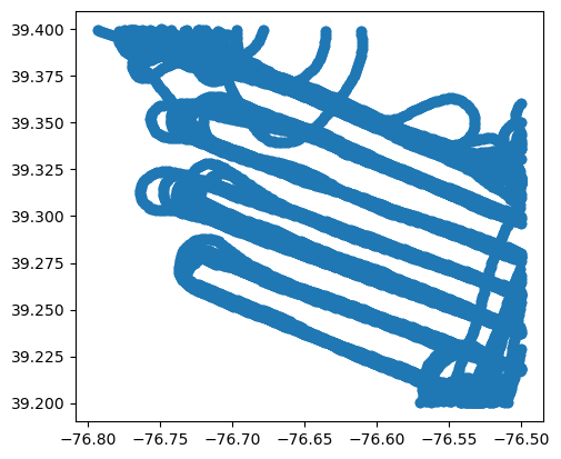
Adjust the latitudes and longitudes in the box() call below to profile a different spatial area. Format for the bounding box is: (West, South, East, North).

# clip data to just the region around baltimore
bbox = box(-76.8, 39.2, -76.5, 39.4)  # latitude and longitude of the bounding box
b200_baltimore = gpd.clip(b200, mask=bbox)

b200_baltimore.plot()

<Axes: >

The cell below shows how to use the .explore() function to create an interactive map for viewing where the data has been collected. This is a processing intensive function, so a few notes about using it:

1. Careful running this on more than ~50,000 rows of data. The map may run very very slowly

2. You may need to re-start your kernel if you run the line multiple times. The memory can fill up quickly

b200_baltimore.explore(column='NO2_CANOE_STCLAIR')

Make this Notebook Trusted to load map: File -> Trust Notebook

Code Summary: Preprocessing

Divide the data into bins and filter to just the \(NO_2\) data.

# Create a dataframe of only NO2 and altitude
no2 = b200_baltimore[['NO2_CANOE_STCLAIR', 'gpsALT_ft_THORNHILL']]
# Make an array from 0 feet to 11,000 feet with jumps of 250 feet in between
bins = np.arange(0, 11_000, 250)
# Create a label for each row of which bin it is in
height_groups = pd.cut(no2['gpsALT_ft_THORNHILL'], bins)
# Group the data by bin
binned_no2 = no2.groupby(height_groups).mean()['NO2_CANOE_STCLAIR'].reset_index()

/tmp/ipykernel_2336/2763294332.py:8: FutureWarning: The default of observed=False is deprecated and will be changed to True in a future version of pandas. Pass observed=False to retain current behavior or observed=True to adopt the future default and silence this warning.
  binned_no2 = no2.groupby(height_groups).mean()['NO2_CANOE_STCLAIR'].reset_index()

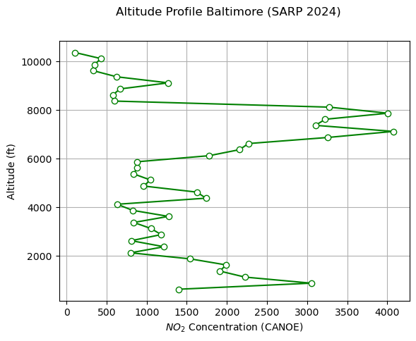
Code Summary: Plotting

# Define the midpoint altitude for each bin
bin_centers = binned_no2['gpsALT_ft_THORNHILL'].apply(lambda x: x.mid)

fig, ax = plt.subplots()

# Add data
ax.plot(binned_no2['NO2_CANOE_STCLAIR'], bin_centers, 'g-o', 
        markerfacecolor='white')

# Add x and y axis labels
ax.set_xlabel('$NO_2$ Concentration (CANOE)')
ax.set_ylabel('Altitude (ft)')

# Add gridlines
ax.grid()

fig.suptitle('Altitude Profile Baltimore (SARP 2024)')

Text(0.5, 0.98, 'Altitude Profile Baltimore (SARP 2024)')